FAKE NEWS CHALLENGE

Richard Godden

[email protected]

github.com/goddenrich

Oriana Fuentes

[email protected]

github.com/fuentesori

Jonathan Chan

[email protected]

github.com/jchanaf

Killian Robert Rutherford

[email protected]

github.com/killianrutherford

Abstract

Fake news has recently risen to the forefront of society due to its perceived influence on recent political events. The problem of discerning fact from fiction is by no means new, however we find ourselves at a point in history where we have enough data from connected sources on the internet to start to tackle the challenge using machine learning. The Fake news challenge[1] was established to explore how machine learning and AI techniques could be employed to automate the current manual, fact checking process. The organizers of the challenge have provided a baseline which uses hand crafted features designed specifically for the task. We would like to explore techniques using pretrained word2vec[2][3] embeddings and not use hand crafted features. We have shown many methods can be applied to this task including ensemble methods and recurrent neural networks. We found that it was possible to beat the baseline focusing on SVD and Bag of Words models to fit into SVM classifiers.

1. Introduction

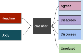
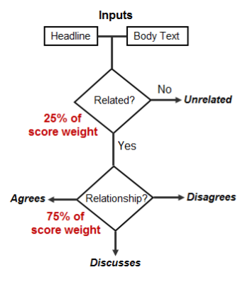
The Fake News Challenge was established to explore how machine learning and AI techniques could be employed to automate the, current manual, fact checking process. This process is a complex pipeline which can be broken down into subtasks. The first step in this process is to identify articles that support or refute a claim. To do this we have to determine stance, validity and association between texts. The challenge is to determine the stance of two pieces of text to a topic, claim or issue. The organizers chose the task of determining the stance between an excerpt from a news article and a headline to determine whether the headline and body agree, disagree, discuss or are unrelated to each other.

Fig 1.1 The classification task                                 Fig 1.2 The scoring mechanism

The 4 classes have been defined as follows:

1. Agrees: The body text agrees with the headline
2. Disagrees: The body text disagrees with the headline
3. Discusses: The body text discusses the same topic as the headline, but does not take a position
4. Unrelated: The body text discusses a different topic than the headline

The task of deciding whether a body  is unrelated or related to a headline is a much easier task than deciding on the three other classifications. To reflect this, the scoring mechanism gives more weight towards correctly identifying whether an article agrees, disagrees or discusses rather than identifying unrelated header and bodies [1].

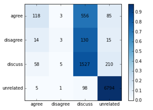
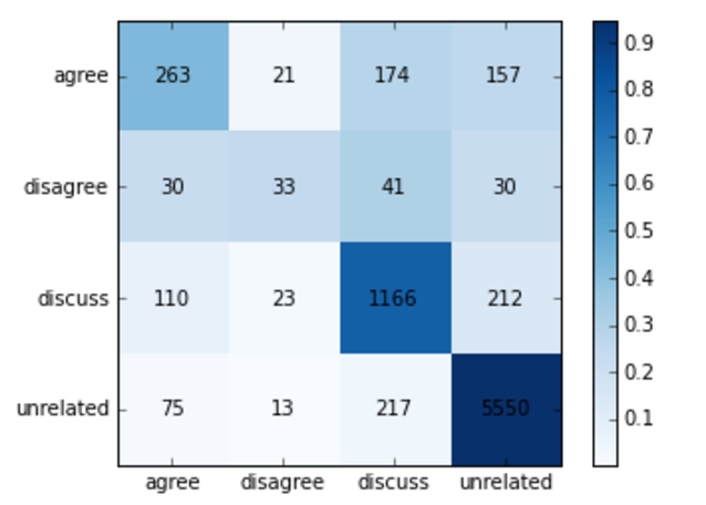
The organisers of the challenge provided a baseline using hand-coded features designed for this task and used a Gradient boosting classifier which obtains a test score (based on the scoring described above) of 79.53%. One issue with the dataset which we will discuss below is that a naive splitting of train and test such that the baseline provides means that articles that appear in the training set will also appear in the test set. We call this bleeding. Without allowing bleeding the baseline obtains a test score of 76.69%.

Fig 1.3 confusion matrix of the baseline model on the bleeded data set. The rows indicate the ground truth labels, and the columns are the model predicted labels. The baseline does a reasonable job of discerning related and unrelated but is not very good at classifying correctly within the related classes.

2. Data

2.1. Fake News Challenge Dataset

The data provided by Fake News Challenge consists of 1,647 unique headlines and 1,682 unique articles bodies. These are associated with each other and then tagged as: agree, disagree, discuss or unrelated. Below is the distribution of the 49,972 associations between the different headlines and bodies:

agree: 3,678
disagree: 840
discuss: 8,909
unrelated: 36,545

As the data stands, it cannot be easily split into test and training for cross-validation purposes due to the fact that headlines are associated across several bodies and vice-versa. When splitting the data naively, bodies or headlines will ‘bleed’ into the test sets as they will have most likely been trained upon already. Additionally, when considering the unique bodies and headlines, rather than the set of associations, we encounter a relatively small sample size.
In order to remedy the ‘bleeding’ of headlines and bodies across training and test sets, we will pick a subset of headlines to train and remove the headlines that are associated with these from the set that will be tested upon. In order to remedy the limited amount of unique bodies and headlines, we will augment the dataset by generating new bodies and headlines with synonyms and related words.

2.2 Data Augmentation

2.2.1 Windowing

In order to produce more data points to train on we split the article bodies into a list of strings. Each window was set to be 150 tokens long and then the window is slided 75 words over. The overlapping window ensures that each window is of a reasonable size so that we didn’t have article bodies with few or singleton words.

2.2.2 Word substitution

Another method that we used to increase the size of the dataset was word substitution of the headlines based on a technique proposed by Vijayaraghavan [4]. We could have run this on the bodies as well, but we were able to generate a dataset magnitudes larger than the original with the windowing and word substitution on headlines strategy. For a given headline, we select target words that are not common stoplist words and are not compound words, which we approximated by checking whether consecutive pairs of words in the headline were in the word2vec vocabulary. For each target word, we generated a candidate list of synonyms, hyponyms, hypernyms in the Natural Language Toolkit (NLTK) corpus and then compared the target word2vec representation and the candidate word using cosine similarity, narrowing down the candidates to the 10 with the highest similarity above a certain threshold. We found that .34 was a reasonable threshold. Once we obtained this list of candidate words, we randomly selected target words in each headline and randomly picked words in the candidate list to replace it with. We did this multiple times for each headline in the dataset in order to generated a significantly larger dataset.

3. Methods

3.1 data processing

The original data is processed by data_splitting.py which has a series of tools and methods to handle the different steps of the process shown below:

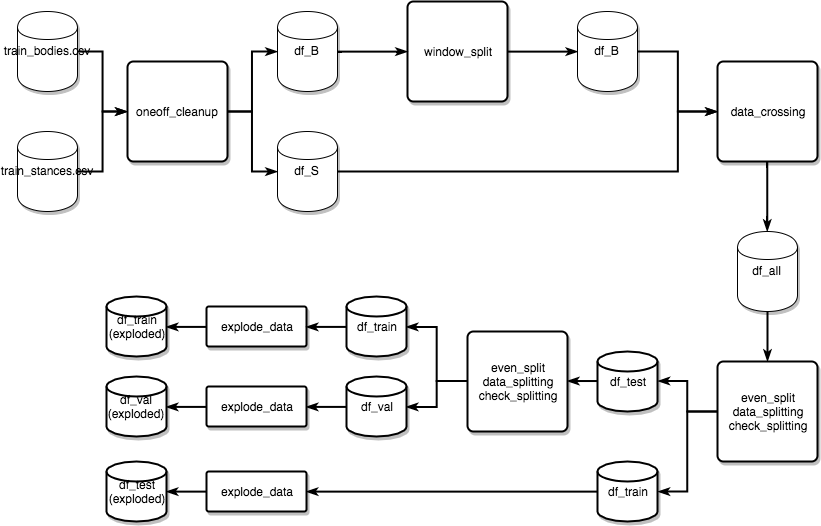
Figure 3.1.1: Flow chart depicts the data processing pipeline

The original .csv files from the challenge, train_bodies and train_stances are passed to data_splitting which runs preprocess_all. The first step is to run import_data and convert the .csv files to pandas dataframes, run oneoff_cleanup which removes only a handful of bodies which are not in english. Then the bodies are passed to window_splitting which splits the bodies into a list of strings with a sliding window of 150 tokens with 75 token overlap. One converted into a list of strings, the bodies and stances are crossed with data_crossing. The function data_crossing will attach the bodies related to the body ids in the stances dataset, and re-indexes the bodies so they can be split by index to create test, training and cross validation sets. At this point a dataframe called df_all is returned which contains the full panel of stances, headlines, and article bodies, along with additional indexing for headlines and bodies in order to split them efficiently and avoid bleeding. The dataframe df_all is passed to even_split which takes a subset of the body IDs and a subset of headline IDs, for example 70% and picks only the associations between those two 70% sets within the list of 49,972 associations. even_split calls data_splitting and check_splitting, which perform the splitting described above and then checks whether the distribution of stances (agree, disagree, etc) is close to the distribution of these in the original data. The dataframes are then saved into .csv files.

3.2 Ensemble methods

The initial problem was, given the 300 state space word2vec (w2v) representation mentioned above, to reconstruct a representation of the header and body paragraphs. Several ideas were attempted, and fed into a variety of ensemble methods, with results detailed in the next section. All tests were conducted on non-bleeded datasets to attempt to obtain as accurate representations of the data as possible.

3.2.1 SVD

The initial preprocessing step involved creating a matrix of vectors to represent the body and header paragraphs. For each word found in the w2v model, a vector was concatenated to the header/body matrix, to give a final matrix representation of each paragraph with dimensions (300, #valid words).

Standard kSVD was applied to each header and body matrix to obtain the top k eigenvector representatives of the header/body. Primarily dealing with the top eigenvector, as well as the average of top k eigenvectors, cosine similarity was compared between header and body to attempt to identify linear ranges between the four classes: unrelated, discuss, agree, disagree. Although this gave some sort of indication as to whether the header and body were related, it did not yield conclusive results on a four-way classification, with predictions between agree, disagree, and discuss rarely performing better than random.

3.2.2 SVM and Ensemble

Given the top eigenvector (ranked by decreasing value of eigenvalue) for header and body, this could be fed into a specific method as a feature vector.

Concatenation and subtraction of header-body eigenvectors were attempted, (600 and 300 feature vector respectively); a hyperparameter grid search was conducted over a variety of different methods and method parameters to obtain the results in section 4.1.1.

3.2.3 Bag of Words

Following a method proposed by [5], stop words are primarily not included in any of the above matrix representations for header and body. The body is split up into its respective sentences, and each sentence is represented by an average word vec of words in that sentence. The average head word vector is then calculated for these matrices, and cosine similarities of all the body sentence word vectors and the average head word vec are compared. The three body sentence word-vectors with the highest cosine similarity are concatenated, along with the average head vector and fed into a classifier (dimension of 1200).

This bag of words method in the original paper boasted high score metrics (in the 80 percents). Taking some of the top performing ensemble methods from the previous section, different hyperparameters were experimented with, as well as the number of sentence vectors to be concatenated. As can be seen in section 4.1.2 some of our best scores were able to be retrieved.

3.2.4 Penalty and Augmentation

In an attempt to incorporate ideas from previous sections, the final outlook on the problem involved mixing SVD eigenvectors and average word vectors together. The top eigenvector and average vector for both header and body were concatenated together to give a feature vector of size (1200). The training data was primarily augmented by splitting each body paragraph into two and assigning the same class with headers.

In addition to this, we incorporated various ideas of feature selection involving L1 penalties learnt in linear LASSO methods to these non-linear situations. However, feature selection given non-linear kernel SVM’s has always proven to be hard. Although some methods have been performed, using attempts such as hybrid recursive feature extraction algorithms, we leave such complicated recursive implementations for further improvement work [6].

Instead, we first feature-select using tree based methods, and trim the input data to include only relevant features, before passing it into the the best performing classifiers above, namely polynomial and RBF kernel SVM as well as KNN (see results in 4.1.3).

The final trials on the data involved solely focusing on svm polynomial kernel (which has consistently been the most performant model). A larger hyperparameter grid search was performed to select the best model parameters:  

Following this, a more sophisticated data augmentation method of windowing as described in previous data augmentation sections was utilised and applied both to the above concat/average mixed method, and the stanford bag of words model as well as incorporating feature selection, although this did not improve the performances that were already achieved up until this stage.

3.3 LSTM models

An approach with which to compare the above are neural networks. This would not require feature extraction. However, networks typically require a large amount of data to produce accurate results; to this end, we will augment the data as described above. This task is a sequence to label task and one appropriate model to handle these types of tasks is using recurrent neural networks and in particular long short term memory networks or LSTMs are adept to reasoning about over long dependent series. We decided to implement two versions of these networks that have been successful. One a bidirectional LSTM and in the other case, we add an attention layer which allows us to learn a weighting between the LSTM states at different points in the headline and in the body.

3.3.1 Bidirectional LSTM

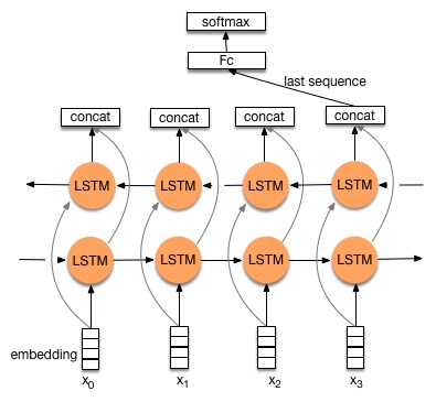
A standard LSTM classifier was implemented using 100 hidden units and a 512 unit softmax classification layer as the baseline deep learning model. The LSTM cell is calculated with the usual input, forget, cell, and output states. The first is a bidirectional LSTM where the input data is read forwards by one layer of LSTM units and in reverse order by another layer of LSTM units. The outputs of each direction are concatenated before being used.

Fig 3.3.1.1 visualization of the bidirectional lstm model [7]

3.3.2 Bidirectional LSTM with attention

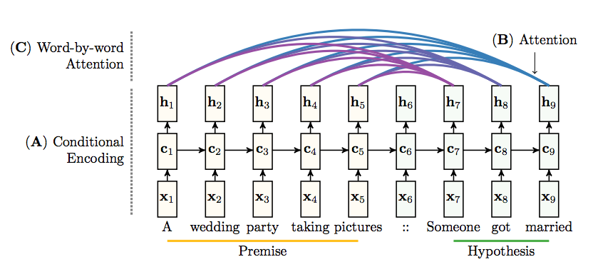
Previous work has been done in a similar problem, determining entailment, involving conditioning Long Short-Term Memory networks by Rocktaschel [8]. The entailment problem is understanding whether 2 sentences: entail each other, disagree with each other, or are unrelated. Their approach encodes each sentence using Word2Vec and passes each of them to separate LSTMs, with a slight modification. One of the LSTMs initializes the hidden state of the other LSTM with the last output of its hidden state. With this conditional encoding technique, they achieved 80% accuracy on the test set of Stanford Natural Language Inference corpus.

Fig 3.3.2.1 visualization of the LSTM model with attention [8]

One challenge with the Fake News Challenge that neither the LSTM nor the bidirectional conditioned global attention LSTM approach handles is that the problem compares a sentence with a body of sentences. To address this, we had two approaches. In one, we simply limited the number of word2vec tokens in the body to 150. The other approach was to split the body of sentences into 150 word2vec tokens by running a sliding window across the body, feeding these with their respective headline to the neural network.

4. Results 

4.1. Ensemble

4.1.1 SVM and Ensemble Methods

Preliminary results from hyperparameter and ensemble grid search using only top eigenvector from header and body gave the following: (The score percentage is measured according to the Fake News Challenge scoring [1]). (60/40 train/test and cross-validation used).

Table 1: Initial Hyperparameter Search Ensemble Methods for Subtraction and Concatenation of Header/Body SVD Eigenvectors

Interesting results can be seen, with greater testing accuracies and scores achieved with SVM’s with RBF and Polynomial kernels, and K Nearest Neighbours. Although RBF SVM’s seem to perform better for subtraction of eigenvectors, the final best result is with polynomial kernel SVM’s with concatenation. This result of 65.8% is not nearly as good as the baseline model, which on the same non-bleeded datasets gives a performance of around 76.7%. However, given the simplicity of taking top SVD eigenvectors compared to the complex hand crafted features of the baseline models, these results give a promising first step.

4.1.2. Bag of Words

Taking the best performing models from the previous section, we attempt to fit the Bag of Words  (BOW) model, monitoring and varying the number of top eigenvectors taken to feed into the classifier. The best results for each classifier are displayed below (with a 60/40 train/test split and cross-validation used).

Table 2: Bag of Words Model for Ensemble Methods

We see some very good results from this result, in fact improving over the baseline model by about 3 percent, without needing any hand crafted features whatsoever. This demonstrates a certain impressive conclusion regarding the properties of the word2vec model, in terms of how representative of a text the top 3 or even top 1 similar average sentence vectors are to the header.

Fig 4.1.2 Bag of Words 86.41% accuracy and a total score of 79.20%. The rows indicate the ground truth labels, and the columns are the model predicted labels.

As can be seen from the heat map, most classes are heavily classified correctly, although the most issues occur in the agree and disagree classes, most likely due to the lower number of training samples.

4.1.3 Concat augment split half, penalisation feature selection

Mixing previous models, by concatenating the average word to vec and top eigenvector for header and bodies, as well as adding feature-selection and augmenting the data by splitting the bodies in half, we can retrieve very similar results to the BOW Model.

Table 3: Mixture of Average and SVD Eigenvector Concatenation with Feature Selection

Interestingly, the KNN model performs better than in the BOW model. However, the best result, which comes again from a SVM polynomial kernel is just a very slightly lower score than the BOW model, but performs much better than the baseline.

4.2. LSTM

This section describes the results of the LSTM-based methods discussed in section 3.3. We present the confusion matrices for the baseline LSTM and the bidirectional conditioned global attention LSTM in Fig 4.2.1 and Fig 4.2.2 respectively. The baseline LSTM method had a higher raw accuracy than the bidirectional conditioned global attention LSTM, where accuracy is the unweighted classification accuracy. In contrast, the bidirectional conditioned global attention LSTM had a higher score, as calculated in the Fake News Challenge, which is a weighted classification score.

Looking at the confusion matrix, this difference between accuracy and Fake News Challenge score is more apparent. The baseline LSTM has a tendency towards the majority class Unrelated. Disagree, which is the least represented in the dataset, is rarely predicted. Only 4 were predicted to be disagree out of 7536. While the bidirectional conditioned global attention LSTM had a lower accuracy, the model predicted a higher proportion of classes that were not unrelated, resulting in a higher score.

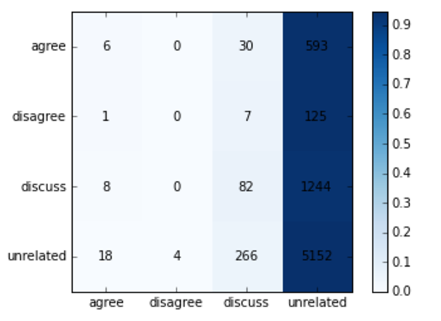
Fig 4.2.1 Baseline LSTM Confusion Matrix for the test set, resulting in 70% accuracy and a total score of 40.1. The rows indicate the ground truth labels, and the columns are the model predicted labels.

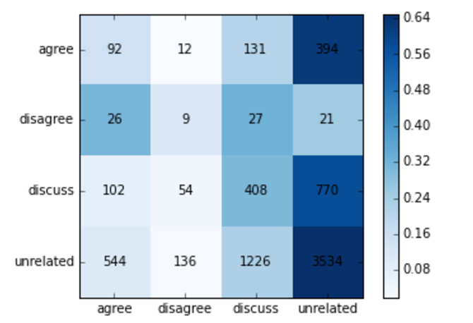
Fig 4.2.2 Bidirectional Conditioned Global Attention LSTM Confusion Matrix for the test set, resulting in 54% accuracy and a total score of 42.8. The rows indicate the ground truth labels, and the columns are the model predicted labels.

5. Conclusions and next steps

    We were able to achieve similar results and in some cases beat the baseline model using word2vec embeddings to represent words in the texts and training classifiers using various SVD and data manipulation to feed into ensemble methods. The best performing of these involved SVM classifiers, particularly with polynomial kernel, where on a 60/40 train/test split we were able to obtain a score of 79.2% compared to the baseline of 76.7%.

Unfortunately such accuracies were not able to be reproduced with the bidirectional LSTM, although certain interesting properties could be determined from the resulting confusion matrices.

Further work will involve continuing to develop the SVD models to feed into SVM classifiers, including possibly utilising higher order SVD (tensor-SVD) methods (some preliminary work can be found on our github link [0]) as well as look into some more innovative methods to penalise non-linear kernel classifiers. Furthermore, increased efforts will be made towards tuning the bidirectional LSTM to attempt to obtain higher accuracies before submission to the competition.

6. References

[0] Our code can be found in the following repository on github:github.com/goddenrich/AML 

[1] D. Pomerleau and D. Rao, “Fake news challenge.”www.fakenewschallenge.org/ GitHub github.com/FakeNewsChallenge 

[2] Tomas Mikolov, Kai Chen, Greg Corrado, Jeffrey Dean Efficient Estimation of Word Representations in Vector Space arXiv:1301.3781 [cs.CL] URL arxiv.org/pdf/1301.3781.pdf 

[3] drive.google.com/file/d/0B7XkCwpI5KDYNlNUTTlSS21pQmM 

[4] Prashanth Vijayaraghavan, Ivan Sysoev, Soroush Vosoughi and Deb Roy DeepStance at SemEval-2016 Task 6: Detecting Stance in Tweets Using Character and Word-Level CNNs arXiv:1606.05694 [cs.CL] arxiv.org/abs/1606.05694 

[5] Mrowca, D., Wang, E., Kosson, A. Stance Detection for Fake News Identification. URL  web.stanford.edu/class/cs224n/reports/2760496.pdf 

[6]  Liu Q. et al. Feature selection for support vector machines with RBF kernel. Artificial Intelligence Review 36(2):99-115 August 2011. URL  www.researchgate.net/publication/220637867_Feature_selection_for_support_vector_machines_with_RBF_kernel 

[7] www.paddlepaddle.org/doc/demo/sentiment_analysis/sentiment_analysis.html 

[8] Tim Rocktäschel, Edward Grefenstette, Karl Moritz Hermann, Tomáš Kočiský, Phil Blunsom Reasoning about Entailment with Neural Attention arXiv:1509.06664 [cs.CL] arxiv.org/abs/1509.06664